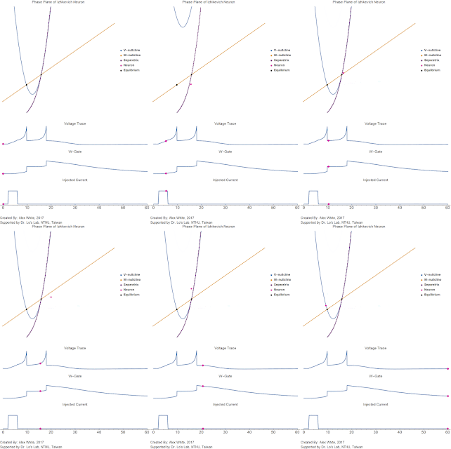
The mathematics of bistability.

Bistability is the coexistence of two different attractors. Normally it is thought as two different stable equilibria separated by an unstable equilibrium (or saddle points). This can give rise to a wide variety of different functions, such as up and down states ,  NMDA spikes, and found in the Izhikevich model. Furthermore, bistability plays a important role in networks of neurons, especially decision networks. Given that bistability is so important in neuroscience (as well as other fields) I wanted to go over the mathematics of bistable systems, and really focus on the mathematics, not the neuroscience.

To begin, bistability is two stable attractors coexisting at the same time. Often we look at two equilibrium. The most simple example of a bistable differential equation is

\begin{equation}
\frac{dx}{dt}= x-x^3
\end{equation}
and I have plotted a graph of $x$ versus $\frac{dx}{dt}$ below. As we can see the system has a characteristic cubic curve that creates three equilibrium points. By setting
\begin{equation}
0=\frac{dx}{dt}= x-x^3
\end{equation}
we quickly find that we have three equilibrium points $x=-1$, $x=0$, and $x=+1$. We can calculate the Jacobian at each of these points. and quickly find that the eigenvalues are


\begin{equation}
\frac{\partial\frac{dx}{dt}}{\partial x}=1 - 3 x^2
\end{equation}
giving us $\lambda = -2$ at $x=\pm1$, $\lambda = +1$ at $x=0$.
Thus we see the system has two stable equilibrium and one unstable equilibrium. Because this system is one-dimensional the unstable equilibrium is our separatrix, and separates our two attractors. In the graph below I have a fifty different initial conditions and I allow them settle down to whichever attractor they want. As you can see all the initial conditions below the separatrix go towards $x=-1$, and all the points above the separatrix go towards $x=+1$. Thus, or separatrix separates the system into two different basins of attraction.

Top: 50 different initial conditions each with their own color. As time progresses the solutions approach the equilibrium point in their basin of attraction. The one solution that starts on the unstable equilibrium stays on the unstable equilibrium. Bottom: The graph of x and $\frac{dx}{dt}$.

However, there is more that we can consider. Imagine we can shift the curve up and down with some constant $k$, as in the GIF below.  As we raise the value of $k$ we can see that there is a saddle-node bifurcation of the negative equilibrium point resulting in a single equilibrium, resulting in a monostable system (one attractor). Likewise, if we decrease $k$ there is a saddle-node bifurcation for the other attractor. Furthermore if we allow $k(t)=2 \sin(\omega t)$ to be a function of time, we can actually force the system and change which attractor it is in.
$$
\frac{dx}{dt}= x-x^3+ k
$$

One important thing to note here, is the value of $k$ that causes this saddle-node bifurcation. This is fairly easy to calculate in the 1-D case. We begin by noting that a saddle-node bifurcation occurs when two equilibria points (the stable and unstable) collide with one another. It is easy to see that this will occur when the local extrema touches the x-axis. Furthermore, because it also happens to be the point when the derivative $\frac{\partial\frac{dx}{dt}}{\partial x}=0$, and satisfies the non-hyperbolicity condition i.e. the system has a single eigenvalue that equals $0$.

Top: 50 different initial conditions each with their own color. Here we let $k=\sin( t/2 )$, this cause successive saddle node bifurcations and force all solutions to converge. However, because of the periodic forcing the solutions do switch between the up and down state.  The black circle is the unstable equilibrium point. Bottom: The graph of x and $\frac{dx}{dt}$. I have slowed down time in the bottom graph so  one can see the convergence better.

We can use this fact that the saddle-node bifurcation point will occur when the eigenvalue of one of the equilibrium points equal to zero, and use that information to solve for $k$.

Thus we get the system:
$$ 0 = x-x^3+ k $$
$$\frac{\partial\frac{dx}{dt}}{\partial x}=0 = 1- 3 x^2 $$

We use the bottom equation to find that the bifurcation point will occur at $ x = \pm \sqrt{\frac{1}{3}} $.
Then we can plug that into the top equation to find the value of $k = \pm(\sqrt{\frac{1}{27}}-\sqrt{\frac{1}{3}}) $. Thus any $k$ with absolute value above $k>|(\sqrt{\frac{1}{27}}-\sqrt{\frac{1}{3}})|$ is sufficient to turn the bistable system into a monostable system. This is how most bistable systems are turned into useful computational devices. Momentarily destroying the bistability in order to drive the system into the desired attractor, which is the primary way decision networks work. Furthermore,  if this looks a lot like the Fitzhugh Nagumo model, that is because relaxation oscillators like these are, bistable systems with a 2nd slow variable acting, usually $w(t)$ or $u(t)$, as the $k=\sin( \omega t)$. We used above. For more info on relaxation oscillators see here, and here.

To conclude, bistability is clearly important in neuroscience. Understanding these simple computational models, both geometrically and algebraically, is key to finding bistabilities hidden in systems much more complex than these.


Author: Alexander White